0 Introduction
Deep learning researchers have been constructing skyscrapers in recent years. Especially, VGG nets and GoogLeNet have pushed the depths of convolutional networks to the extreme. But questions remain: if time and money aren't problems, are deeper networks always performing better? Not exactly.
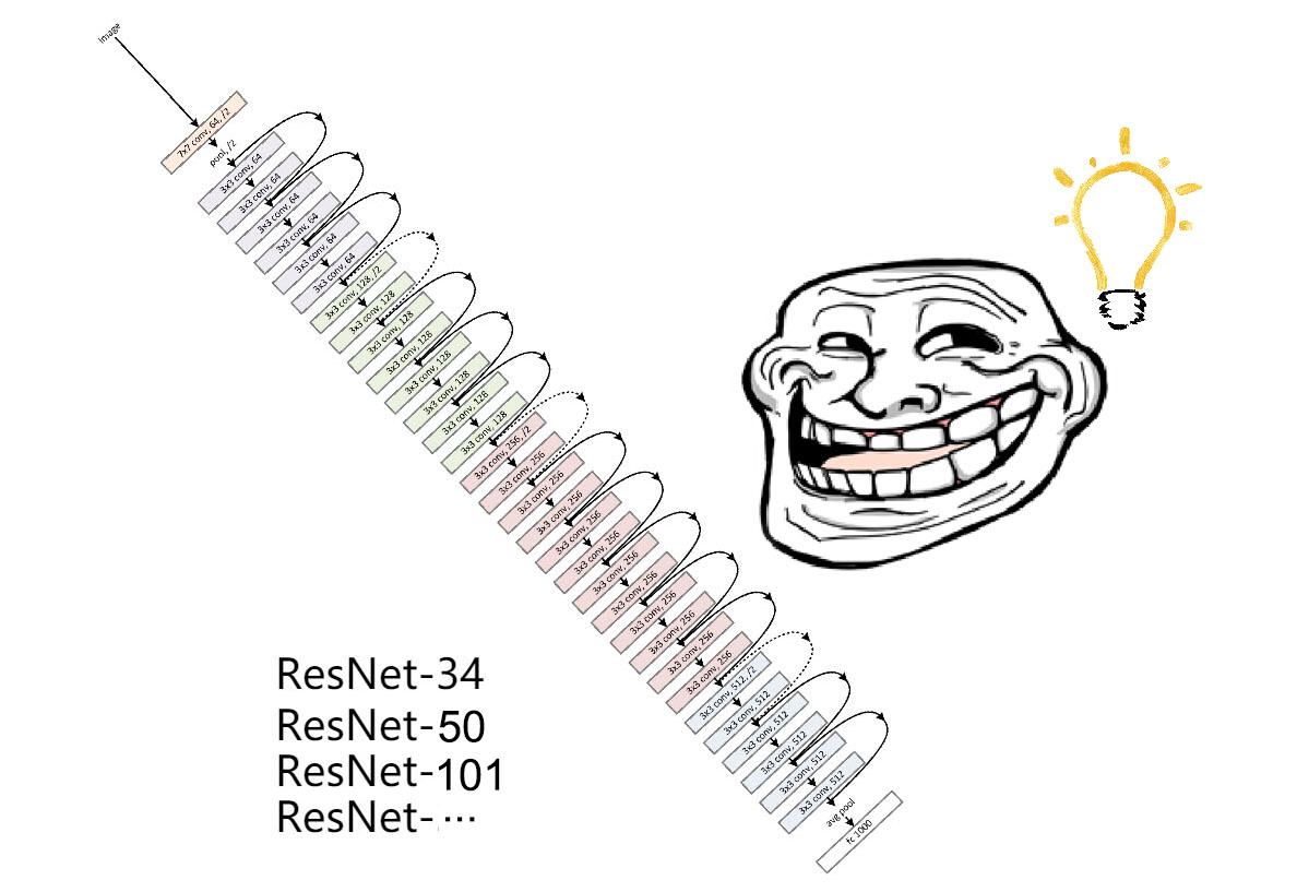
When residual networks were proposed, researchers around the world was stunned by its depth. "Jesus Christ! Is this a neural network or the Dubai Tower?" But don't be afraid! These networks are deep but the structures are simple. Interestingly, these networks not only defeated all opponents in the classification, detection, localization challenges in ImageNet 2015, but were also the main innovation in the best paper of CVPR2016.
1 The Crisis: Degradation of Deep Networks
VGG nets proved the beneficial of representation depth of convolutional neural networks, at least within a certain range, to be exact. However, when Kaiming He et al. tried to deepen some plain networks, the training error and test error stopped decreasing after the network reached a certain depth(which is not surprising) and soon degraded. This is not an overfitting problem, because training errors also increased; nor is it a gradient vanishing problem, because there are some techniques(e.g. batch normalization[4]) that ease the pain.
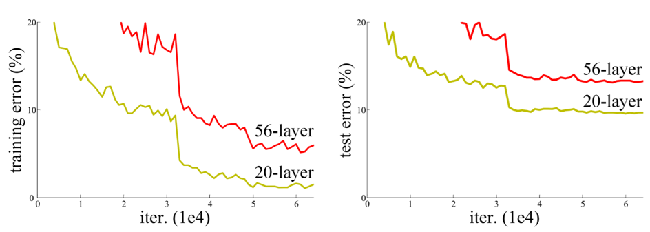
Fig.1 The downgrade problem
What seems to be the cause of this degradation? Obviously, deeper neural networks are more difficult to train, but that doesn't mean deeper neural networks would yield worse results. To explain this problem, Balduzzi et al.[3] identified shattered gradient problem - as depth increases, gradients in standard feedforward networks increasingly resemble white noise. I will write about that later.
2 A Closer Look at ResNet: The Residual Blocks
As the old saying goes, "千里之行,始于足下". Although ResNets are as deep as a thousand layers, they are built with these basic residual blocks(the right part of the figure).
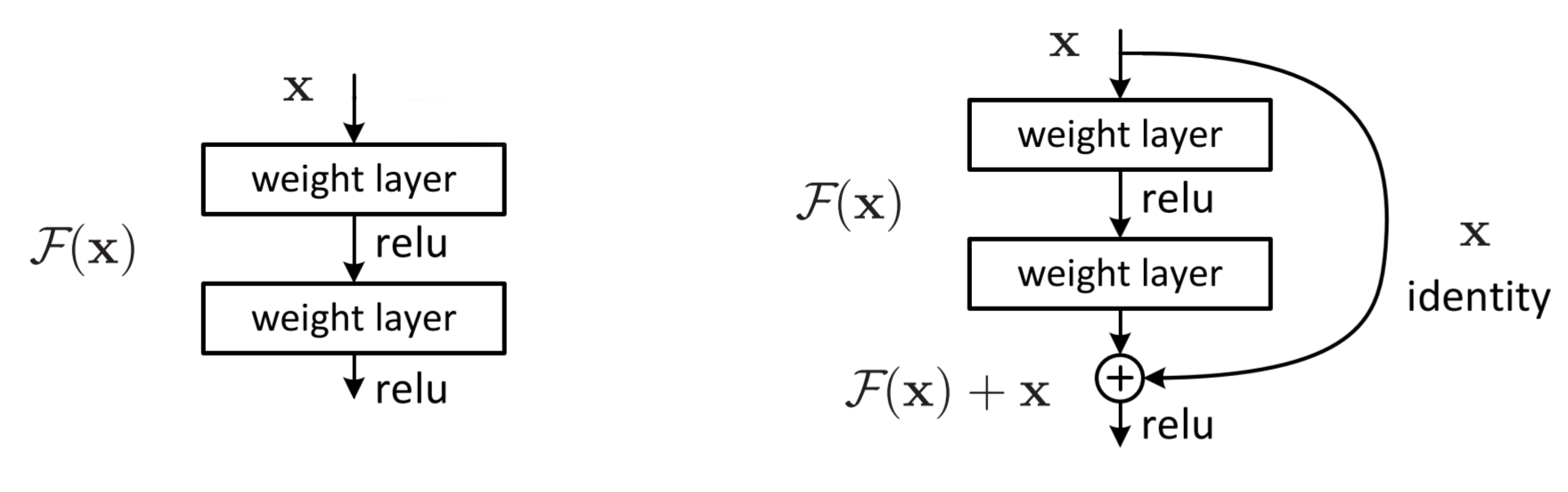
Fig.2 Parts of plain networks and a residual block(or residual unit)
2.1 Skip Connections
In comparison, basic units of plain network models would look like the one on the left: one ReLU function after a weight layer(usually also with biases), repeated several times. Let's denote the desired underlying mapping(the ideal mapping) of the two layers as \(\mathcal{H}(x)\), and the real mapping as \(\mathcal{F}(x)\). Clearly, the closer \(\mathcal{F}(x)\) is to \(\mathcal{H}(x)\), the better it fits.
However, He et al. explicitly let these layers fit a residual mapping instead of the desired underlying mapping. This is implemented with "shortcut connections", which skip one or more layers, simply performing identity mappings and getting added to the outputs of the stacked weight layers. This way, \(\mathcal{F}(x)\) would not try to fit \(\mathcal{H}(x)\), but \(\mathcal{H}(x)-x\). The whole structure(from the identity mapping branch, to merging the branches by the addition operation) are named "residual blocks"(or "residual units").
What's the point in this? Let's do a simple analysis. The computation done by the original residual block is: $$y_l=h(x_l)+\mathcal{F}(x_l,\mathcal{W}_l),$$ $$x_{l+1}=f(y_l).$$
Here are the definitions of symbols:
\(x_l\): input features to the \(l\)-th residual block;
\(\mathcal{W}_{l}={W_{l,k}|_{1\leq k\leq K}}\): a set of weights(and biases) associated with the \(l\)-th residual unit. \(K\) is the number of layers in this block;
\(\mathcal{F}(x,\mathcal{W})\): the residual function, which we talked about earlier. It's a stack of 2 conv. layers here;
\(f(x)\): the activation function. We are using ReLU here;
\(h(x)\): identity mapping.
If \(f(x)\) is also an identity mapping(as if we're not using any activation function), the first equation would become:
$$x_{l+1}=x_l+\mathcal{F}(x_l,\mathcal{W}_l)$$
Therefore, we can define \(x_L\) recursively of any layer:
$$x_L=x_l+\sum_{i=l}^{L-1}\mathcal{F}(x_i,\mathcal{W}_i)$$
That's not the end yet! When it comes to the gradients, according to the chain rules of backpropagation, we have a beautiful definition:
$$\begin{split}
\frac{\partial{\mathcal{E}}}{\partial{x_l}} & = \frac{\partial{\mathcal{E}}}{\partial{x_L}}\frac{\partial{x_L}}{\partial{x_l}}\\
& = \frac{\partial{\mathcal{E}}}{\partial{x_L}}\Big(1+\frac{\partial{}}{\partial{x_l}}\sum_{i=l}^{L-1}\mathcal{F}(x_i,\mathcal{W}_i)\Big)
\end{split}$$
What does it mean? It means that the information is directly backpropagated to ANY shallower block. This way, the gradients of a layer never vanish or explode even if the weights are too small or too big.
2.2 Identity Mappings
It's important that we use identity mapping here! Just consider doing a simple modification here, for example, \(h(x)=\lambda_lx_l\)(\(\lambda_l\) is a modulating scalar). The definition of \(x_L\) and \(\frac{\partial{\mathcal{E}}}{\partial{x_l}}\) would become:
$$x_L=(\prod_{i=l}^{L-1}\lambda_i)x_l+\sum_{i=l}^{L-1}(\prod_{j=i+1}^{L-1}\lambda_j)\mathcal{F}(x_i,\mathcal{W}_i)$$
$$\frac{\partial{\mathcal{E}}}{\partial{x_l}}=\frac{\partial{\mathcal{E}}}{\partial{x_L}}\Big((\prod_{i=l}^{L-1}\lambda_i)+\frac{\partial{}}{\partial{x_l}}\sum_{i=l}^{L-1}(\prod_{j=i+1}^{L-1}\lambda_j)\mathcal{F}(x_i,\mathcal{W}_i)\Big)$$
For extremely deep neural networks where \(L\) is too large, \(\prod_{i=l}^{L-1}\lambda_i\) could be either too small or too large, causing gradient vanishing or gradient explosion. For \(h(x)\) with complex definitions, the gradient could be extremely complicated, thus losing the advantage of the skip connection. Skip connection works best under the condition where the grey channel in Fig. 3 cover no operations (except the addition) and is clean.
Interestingly, this comfirmed the philosophy of "大道至简" once again.
2.3 Post-activation or Pre-activation?
Wait a second... "\(f(x)\) is also an identity mapping" is just our assumption. The activation function is still there!
Right. There IS an activation function, but it's moved to somewhere else. In fact, the original residual block is still a little bit problematic - the output of one residual block is not always the input of the next, since there is a ReLU activation function after the addition(It did NOT REALLY keep the identity mapping to the next block!). Therefore, in[2], He et al. fixed the residual blocks by changing the order of operations.
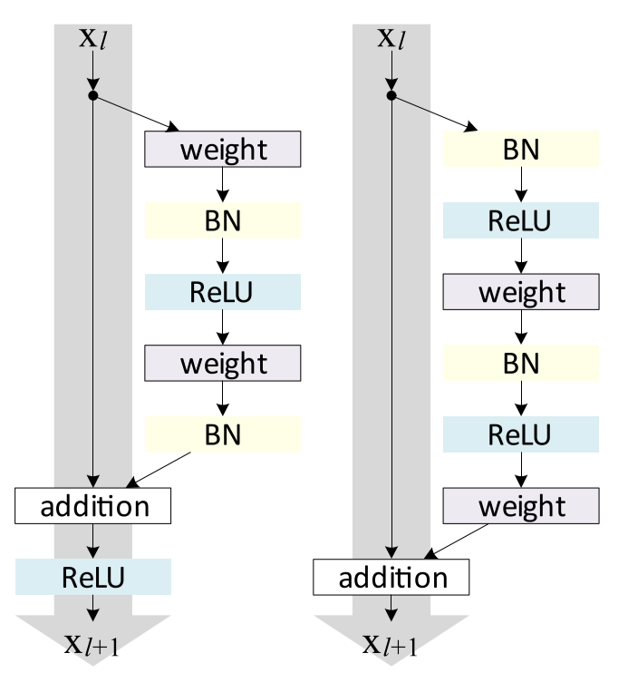
Fig.3 New identity mapping proposed by He et al.
Besides using a simple identity mapping, He et al. also discussed about the position of the activation function and the batch normalization operation. Assuming that we got a special(asymmetric) activation function \(\hat f(x)\), which only affects the path to the next residual unit. Now our definition of \(x_{x+1}\) would become:
$$x_{l+1}=x_l+\mathcal{F}(\hat f(x_l),\mathcal{W}_l)$$
With \(x_l\) still multiplied by 1, information is still fully backpropagated to shallower residual blocks. And the good thing is that using this asymmetric activation function after the addition(partial post-activation) is equivalent to using it beforehand(pre-activation)! This is why He et al. chose to use pre-activation - otherwise it would be necessary to implement that magical activation function \(\hat f(x)\).
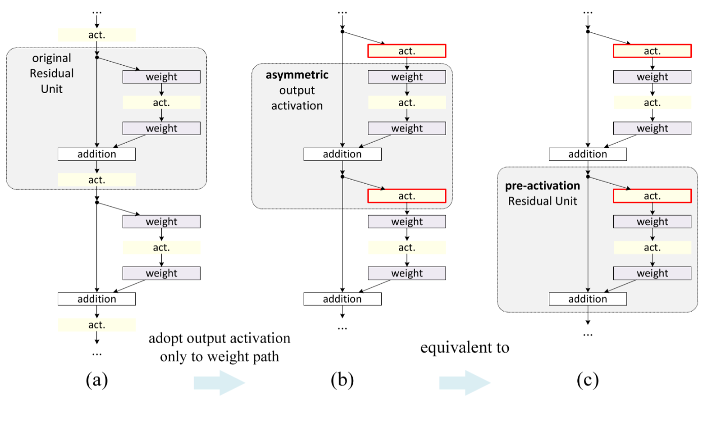
Fig.4 Using asymmetric after-addition activation is equivalent to constructing a pre-activation residual unit
3 ResNet Architectures
Here are the ResNet architectures for ImageNet. Building blocks are shown in brackets, with the numbers of blocks stacked. With the first block of every stack(starting from conv3_x), a downsampling is performed. Each column represents one of the residual networks, and the deepest one has 152 weight layers! Since ResNets were proposed, VGG nets - which were officially called "Very Deep Convolutional Networks" - are not relatively deep anymore. Maybe call them "A Little Bit Deep Convolutional Networks".
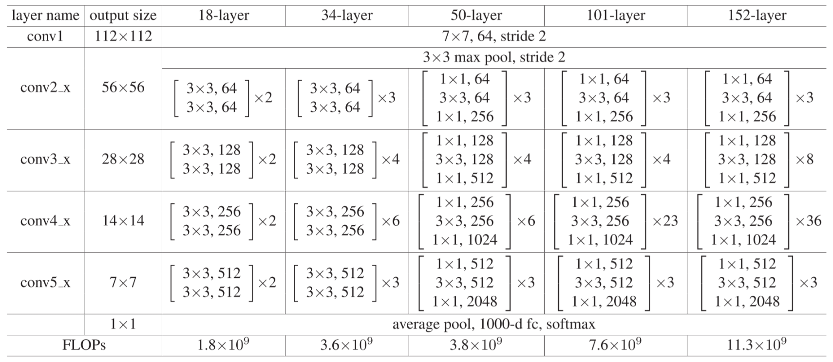
Table. 1 ResNet architectures for ImageNet.
4 Experiments
4.1 Performance on ImageNet
He et al. trained ResNet-18 and ResNet-34 on the ImageNet dataset, and also compared them to plain convolutional networks. In Fig. 5, the thin curves denote training error, and the bold ones denote validation error. The figure on the left shows the results of plain convolution networks(in which the 34-layered ones has higher error rates than the 18-layered one), and the figure on the right shows that residual networks perform better than plain ones, while deeper ones perform better than shallow ones.
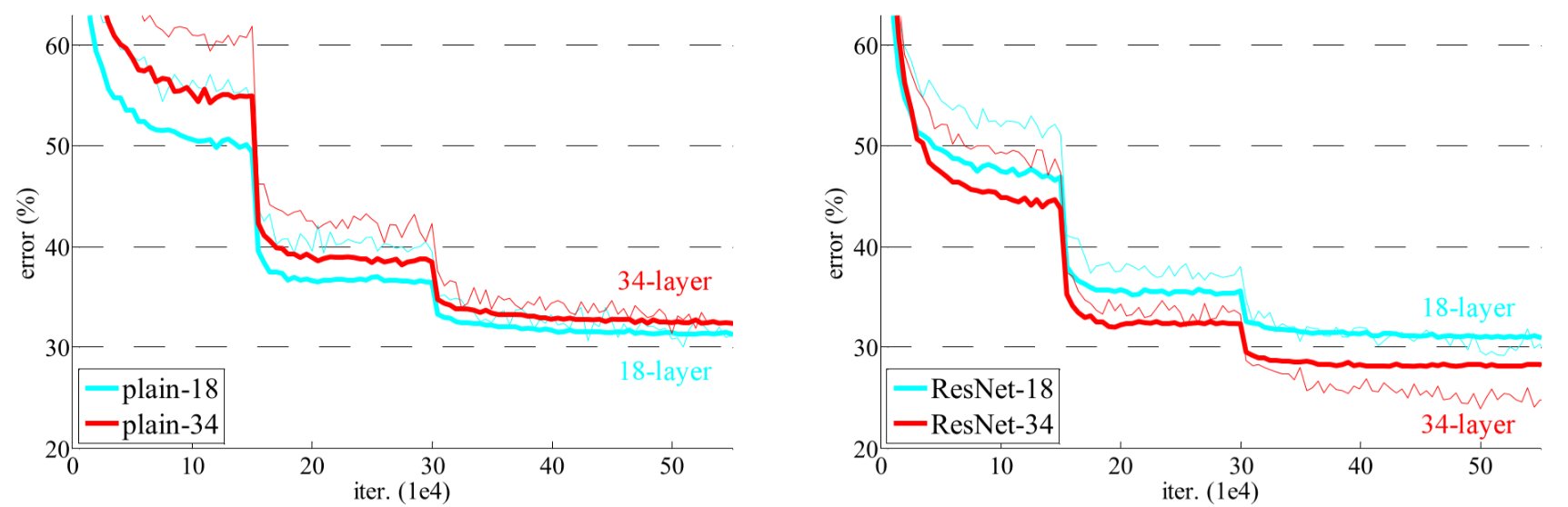
Fig. 5 Training ResNet on ImageNet
4.2 Effects of Different Shortcut Connections
He et al. also tried various types of shortcut connections to replace the identity mapping, and various positions of activation functions / batch normalization. Experiments show that the original identity mapping and full pre-activation yield the best results.
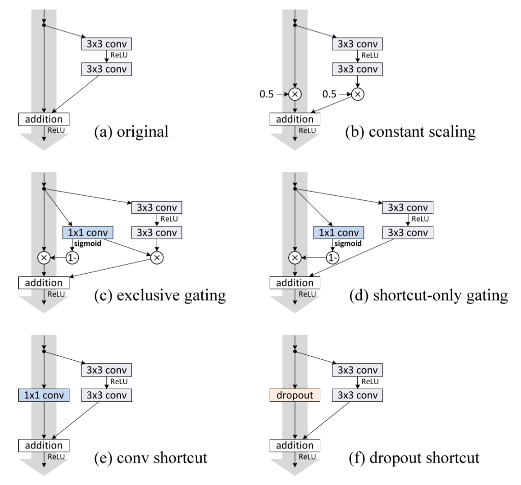
Fig. 6 Various shortcuts in residual units
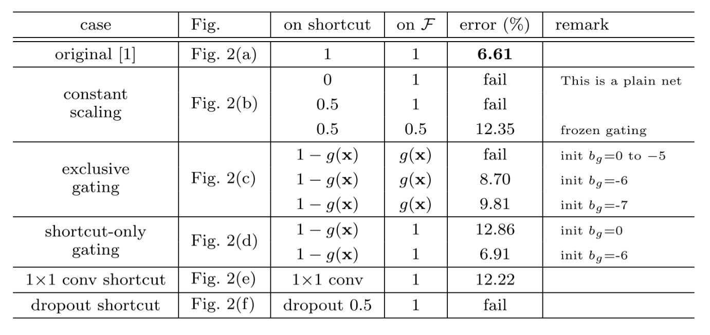
Table. 2 Classification error on CIFAR-10 test set with various shortcut connections in residual units
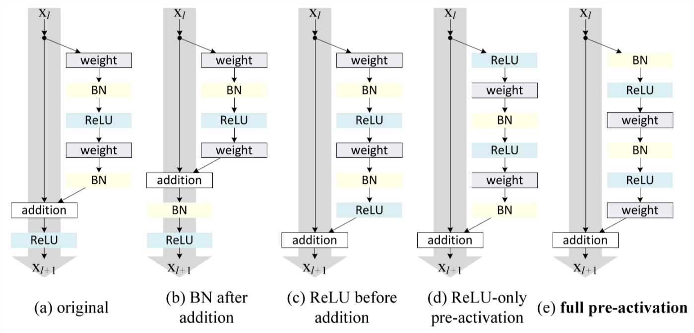
Fig. 7 Various usages of activation in residual units
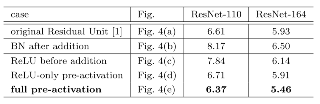
Table. 3 Classification error on CIFAR-10 test set with various usages of activation in residual units
5 Conclusion
Residual learning can be crowned as "ONE OF THE GREATEST HITS IN DEEP LEARNING FIELDS". With a simple identity mapping, it solved the degradation problem of deep neural networks. Now that you have learned about the concept of ResNet, why not give it a try and implement your first residual learning model today?